Downstream analysis on spatial multi-omics data of human gastric cancer
In this tutorial, we will perform downstream analysis of spatial multi-omics data from the human gastric cancer, including identification of MCC flow, group-level MCC, MCC pattern, MCC remodelling in receiver cells.
# Importing packages
import os
import metachat as mc
import numpy as np
import scanpy as sc

import matplotlib.pyplot as plt
from matplotlib import rcParams
rcParams['pdf.fonttype'] = 42
import warnings
warnings.filterwarnings("ignore", category=FutureWarning)
# Setting your work dictionary
os.chdir("/home/project/metachat_packages/")
Import MetaChat results
adata = sc.read('datasets/human_gastric_cancer/metachat_result.h5ad')
Compute group-level MCC of all pairs and all pathways
To summarize MCC patterns between any two group types, we need to compute group-level MCCs across all metabolite–sensor pairs and all pathways.
# extract all_ms_pairs
df_metasen_filtered = adata.uns['df_metasen_filtered']
all_ms_pairs = (df_metasen_filtered['HMDB.ID'] + '-' + df_metasen_filtered['Sensor.Gene']).tolist()
# extract all_metapathways
Metapathway_data = df_metasen_filtered["Metabolite.Pathway"].copy()
Metapathway_list = []
for item in Metapathway_data:
    split_items = item.split('; ')
    Metapathway_list.extend(split_items)
all_metapathways = np.unique(Metapathway_list).tolist()
all_metapathways = [x for x in all_metapathways if x != 'nan']
The original output of MetaChat provides MCC signals for each individual metabolite–sensor pair.
Here, we use mc.tl.summary_communication to summarize the overall MCC activity associated with specific metabolic pathway, aggregating their communication strengths across all corresponding sensors.
mc.tl.summary_communication(adata = adata,
                            database_name = 'MetaChatDB',
                            sum_metapathways = all_metapathways)
Meanwhile, all metabolite–sensor pairs and pathways can be processed together in parallel using the use_parallel=True option. Here, we use the non-spatial version of the statistical test for all metabolite–sensor pairs, since only the group-level MCC scores (rather than p-values) are needed in downstream analyses, allowing faster computation while retaining the same information content.
mc.tl.communication_group(adata = adata,
                          database_name = 'MetaChatDB',
                          group_name = "tissue_type",
                          sum_ms_pairs = all_ms_pairs,
                          n_permutations = 100,
                          use_parallel = True,
                          n_jobs = 100)
Computing group-level MCC: 100%|██████████| 610/610 [00:19<00:00, 31.70it/s]
mc.tl.communication_group_spatial(adata = adata,
                                  database_name = 'MetaChatDB',
                                  group_name = "tissue_type",
                                  sum_metapathways = all_metapathways,
                                  n_permutations = 100,
                                  use_parallel = True,
                                  n_jobs = 100)
Computing group-level MCC: 100%|██████████| 8100/8100 [11:31<00:00, 11.71it/s]
We can first visualize the group-level MCC across all signaling pairs.
fig, ax = plt.subplots(1, 1, figsize=(5,5))
mc.pl.plot_group_communication_heatmap(adata = adata,
                                       database_name = 'MetaChatDB',
                                       group_name = "tissue_type",
                                       cmap = 'red',
                                       permutation_spatial = True,
                                       ax = ax)
ax.set_title('Group-level MCC', fontsize=14)
Text(0.5, 1.0, 'Group-level MCC')
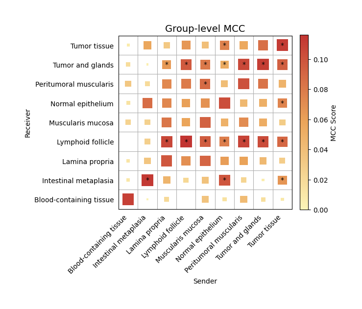
We can observe significant interactions from the tumor tissue toward the surrounding gland regions.
Summary MCC pattern from tumor tissue to glands
In this step, we summarize the MCC pattern specifically from the tumor tissue to the surrounding glands.
By specifying the sender and receiver groups, the mc.tl.summary_pathway function integrates all metabolite–sensor pairs within each pathway and evaluates their overall contributions.
sender_group = "Tumor tissue"
receiver_group = "Tumor and glands"
metapathway_rank, senspathway_rank, ms_result, metapathway_pair_contributions = mc.tl.summary_pathway(
    adata = adata,
    database_name = 'MetaChatDB',
    group_name = "tissue_type",
    sender_group = sender_group,
    receiver_group = receiver_group,
    permutation_spatial = True)
The function mc.tl.summary_pathway() outputs four complementary tables that summarize group-level MCC at multiple biological levels:
• metapathway_rank lists metabolite pathways ranked by their overall communication score, indicating which metabolic routes most contribute to the MCC between the selected sender and receiver groups.
• senspathway_rank ranks sensor-associated signaling pathways by their Rankscore, reflecting how strongly each receptor or signaling cascade is involved in receiving or responding to metabolite-mediated communication.
• ms_result is a matrix showing pairwise communication scores between each metabolite pathway and sensor pathway, capturing how specific metabolic routes couple to particular receptor signaling modules.
• metapathway_pair_contributions provides detailed contributions from individual metabolite–sensor pairs within each metabolite pathway, allowing fine-grained inspection of which molecular interactions drive the observed pathway-level MCC.
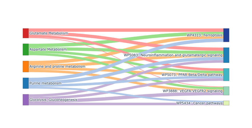
sender_group = "Tumor tissue"
receiver_group = "Tumor and glands"
mc.pl.plot_summary_pathway(ms_result = ms_result,
                           metapathway_rank = metapathway_rank,
                           senspathway_rank = senspathway_rank,
                           plot_metapathway_index = [2,3,5,7,8],
                           plot_senspathway_index = [0,1,3,5,16],
                           figsize = (8,4))
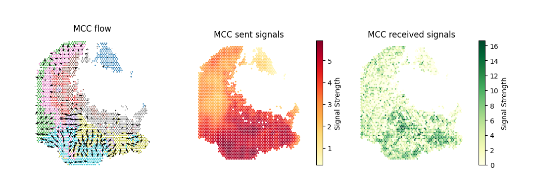
Glycolysis / Gluconeogenesis pathway
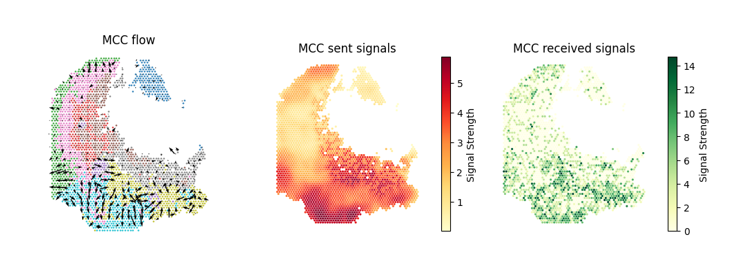
Visualize the spatial distribution of MCC flow and signaling strength for the Glycolysis / Gluconeogenesis pathway.
metapathway_name = "Glycolysis_Gluconeogenesis"
mc.tl.communication_flow(adata = adata,
                         database_name = 'MetaChatDB',
                         sum_metapathways = [metapathway_name],
                         k = 10)
fig, ax = plt.subplots(1, 3, figsize=(12,4))
pl1 = mc.pl.plot_communication_flow(adata = adata,
                                    database_name = 'MetaChatDB',
                                    metapathway_name = metapathway_name,
                                    plot_method = 'grid',
                                    background = 'group',
                                    group_name = 'tissue_type',
                                    summary = 'receiver',
                                    ndsize = 3,
                                    largest_arrow = 0.05,
                                    normalize_v_quantile = 0.995,
                                    grid_density = 0.5,
                                    title = 'MCC flow',
                                    ax = ax[0])
ax[0].set_box_aspect(1)

pl2 = mc.pl.plot_communication_flow(adata = adata,
                                    database_name = 'MetaChatDB',
                                    metapathway_name = metapathway_name,
                                    plot_method = None,
                                    background = 'summary',
                                    group_name = 'tissue_type',
                                    summary = 'sender',
                                    cmap = 'YlOrRd',
                                    ndsize = 5,
                                    largest_arrow = 0.05,
                                    normalize_v_quantile = 0.995,
                                    grid_density = 0.4,
                                    title = 'MCC sent signals',
                                    ax = ax[1])
ax[1].set_box_aspect(1)

pl3 = mc.pl.plot_communication_flow(adata = adata,
                                    database_name = 'MetaChatDB',
                                    metapathway_name = metapathway_name,
                                    plot_method = None,
                                    background = 'summary',
                                    group_name = 'tissue_type',
                                    summary = 'receiver',
                                    cmap = 'YlGn',
                                    ndsize = 5,
                                    largest_arrow = 0.05,
                                    normalize_v_quantile = 0.995,
                                    grid_density = 0.4,
                                    title = 'MCC received signals',
                                    ax = ax[2])
ax[2].set_box_aspect(1)
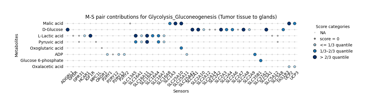
We can use bubble plot to visualize the metabolite–sensor (M–S) pair contributions within the Glycolysis and Gluconeogenesis pathway, focusing on communication from tumor tissue to glands. The bubble size reflects the relative contribution score of each pair, categorized into quantiles of the overall distribution, illustrating which metabolites and sensors are most active in mediating pathway-specific metabolic communication.
pathway_name = "Glycolysis_Gluconeogenesis"
mc.pl.plot_metapathway_pair_contribution_bubbleplot(
    pathway_pair_contributions = metapathway_pair_contributions,
    pathway_name = pathway_name,
    cmap = "blue",
    smallest_size = 10,
    figsize=(12, 3),
    plot_title = f"M-S pair contributions for {pathway_name} (Tumor tissue to glands)"
)
<Axes: title={'center': 'M-S pair contributions for Glycolysis_Gluconeogenesis (Tumor tissue to glands)'}, xlabel='Sensors', ylabel='Metabolites'>
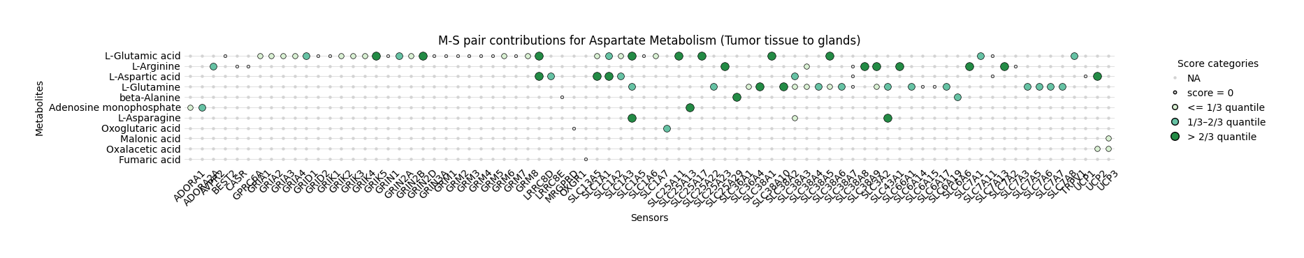
Aspartate Metabolism pathway
Visualize the spatial distribution of MCC flow and signaling strength for the Aspartate Metabolism pathway.
metapathway_name = "Aspartate Metabolism"
mc.tl.communication_flow(adata = adata,
                         database_name = 'MetaChatDB',
                         sum_metapathways = [metapathway_name],
                         k = 10)
fig, ax = plt.subplots(1, 3, figsize=(12,4))
pl1 = mc.pl.plot_communication_flow(adata = adata,
                                    database_name = 'MetaChatDB',
                                    metapathway_name = metapathway_name,
                                    plot_method = 'grid',
                                    background = 'group',
                                    group_name = 'tissue_type',
                                    summary = 'receiver',
                                    ndsize = 3,
                                    largest_arrow = 0.05,
                                    normalize_v_quantile = 0.995,
                                    grid_density = 0.5,
                                    title = 'MCC flow',
                                    ax = ax[0])
ax[0].set_box_aspect(1)

pl2 = mc.pl.plot_communication_flow(adata = adata,
                                    database_name = 'MetaChatDB',
                                    metapathway_name = metapathway_name,
                                    plot_method = None,
                                    background = 'summary',
                                    group_name = 'tissue_type',
                                    summary = 'sender',
                                    cmap = 'YlOrRd',
                                    ndsize = 5,
                                    largest_arrow = 0.05,
                                    normalize_v_quantile = 0.995,
                                    grid_density = 0.4,
                                    title = 'MCC sent signals',
                                    ax = ax[1])
ax[1].set_box_aspect(1)

pl3 = mc.pl.plot_communication_flow(adata = adata,
                                    database_name = 'MetaChatDB',
                                    metapathway_name = metapathway_name,
                                    plot_method = None,
                                    background = 'summary',
                                    group_name = 'tissue_type',
                                    summary = 'receiver',
                                    cmap = 'YlGn',
                                    ndsize = 5,
                                    largest_arrow = 0.05,
                                    normalize_v_quantile = 0.995,
                                    grid_density = 0.4,
                                    title = 'MCC received signals',
                                    ax = ax[2])
ax[2].set_box_aspect(1)
pathway_name = "Aspartate Metabolism"
mc.pl.plot_metapathway_pair_contribution_bubbleplot(
    pathway_pair_contributions = metapathway_pair_contributions,
    pathway_name = pathway_name,
    cmap = "green",
    smallest_size = 10,
    figsize=(18, 3),
    plot_title = f"M-S pair contributions for {pathway_name} (Tumor tissue to glands)"
)
<Axes: title={'center': 'M-S pair contributions for Aspartate Metabolism (Tumor tissue to glands)'}, xlabel='Sensors', ylabel='Metabolites'>
MCC remodelling in receiver cells
In the next step, we aim to identify response genes in receiver cells. To do this, we provide the corresponding raw RNA data (adata_raw) as reference, which allows MetaChat to estimate transcriptional changes associated with signaling activity.
adata_raw = sc.read('datasets/human_gastric_cancer/adata_RNA_raw.h5ad')
Glycolysis / Gluconeogenesis pathway
metapathway_name = 'Glycolysis_Gluconeogenesis'
df_deg, df_yhat = mc.tl.communication_responseGenes(adata = adata,
                                                    adata_raw = adata_raw,
                                                    database_name = 'MetaChatDB',
                                                    metapathway_name = metapathway_name,
                                                    group_name = 'tissue_type',
                                                    summary = 'receiver')
/opt/conda/envs/metachat_test_20251015/lib/python3.9/site-packages/tqdm/auto.py:21: TqdmWarning:

IProgress not found. Please update jupyter and ipywidgets. See https://ipywidgets.readthedocs.io/en/stable/user_install.html

100%|██████████| 100/100 [00:09<00:00, 10.86/s]
  |                                                  | 0 % ~calculating   |+                                                 | 1 % ~08m 26s       |+                                                 | 2 % ~08m 18s       |++                                                | 3 % ~07m 49s       |++                                                | 4 % ~07m 40s       |+++                                               | 5 % ~07m 27s       |+++                                               | 6 % ~07m 18s       |++++                                              | 7 % ~07m 14s       |++++                                              | 8 % ~07m 09s       |+++++                                             | 9 % ~07m 04s       |+++++                                             | 10% ~07m 07s       |++++++                                            | 11% ~07m 01s       |++++++                                            | 12% ~07m 52s       |+++++++                                           | 13% ~07m 42s       |+++++++                                           | 14% ~07m 33s       |++++++++                                          | 15% ~07m 25s       |++++++++                                          | 16% ~07m 22s       |+++++++++                                         | 17% ~07m 16s       |+++++++++                                         | 18% ~07m 10s       |++++++++++                                        | 19% ~07m 04s       |++++++++++                                        | 20% ~06m 57s       |+++++++++++                                       | 21% ~06m 54s       |+++++++++++                                       | 22% ~06m 48s       |++++++++++++                                      | 23% ~06m 42s       |++++++++++++                                      | 24% ~06m 35s       |+++++++++++++                                     | 25% ~06m 47s       |+++++++++++++                                     | 26% ~06m 41s       |++++++++++++++                                    | 27% ~06m 37s       |++++++++++++++                                    | 28% ~06m 30s       |+++++++++++++++                                   | 29% ~06m 23s       |+++++++++++++++                                   | 30% ~06m 17s       |++++++++++++++++                                  | 31% ~06m 10s       |++++++++++++++++                                  | 32% ~06m 04s       |+++++++++++++++++                                 | 33% ~06m 21s       |+++++++++++++++++                                 | 34% ~06m 14s       |++++++++++++++++++                                | 35% ~06m 09s       |++++++++++++++++++                                | 36% ~06m 02s       |+++++++++++++++++++                               | 37% ~05m 55s       |+++++++++++++++++++                               | 38% ~05m 48s       |++++++++++++++++++++                              | 39% ~05m 42s       |++++++++++++++++++++                              | 40% ~05m 35s       |+++++++++++++++++++++                             | 41% ~05m 29s       |+++++++++++++++++++++                             | 42% ~05m 23s       |++++++++++++++++++++++                            | 43% ~05m 21s       |++++++++++++++++++++++                            | 44% ~05m 15s       |+++++++++++++++++++++++                           | 45% ~05m 09s       |+++++++++++++++++++++++                           | 46% ~05m 02s       |++++++++++++++++++++++++                          | 47% ~04m 58s       |++++++++++++++++++++++++                          | 48% ~04m 51s       |+++++++++++++++++++++++++                         | 49% ~04m 45s       |+++++++++++++++++++++++++                         | 50% ~04m 39s       |++++++++++++++++++++++++++                        | 51% ~04m 33s       |++++++++++++++++++++++++++                        | 52% ~04m 27s       |+++++++++++++++++++++++++++                       | 53% ~04m 21s       |+++++++++++++++++++++++++++                       | 54% ~04m 15s       |++++++++++++++++++++++++++++                      | 55% ~04m 09s       |++++++++++++++++++++++++++++                      | 56% ~04m 03s       |+++++++++++++++++++++++++++++                     | 57% ~03m 58s       |+++++++++++++++++++++++++++++                     | 58% ~03m 52s       |++++++++++++++++++++++++++++++                    | 59% ~03m 46s       |++++++++++++++++++++++++++++++                    | 60% ~03m 41s       |+++++++++++++++++++++++++++++++                   | 61% ~03m 35s       |+++++++++++++++++++++++++++++++                   | 62% ~03m 29s       |++++++++++++++++++++++++++++++++                  | 63% ~03m 24s       |++++++++++++++++++++++++++++++++                  | 64% ~03m 18s       |+++++++++++++++++++++++++++++++++                 | 65% ~03m 12s       |+++++++++++++++++++++++++++++++++                 | 66% ~03m 07s       |++++++++++++++++++++++++++++++++++                | 67% ~03m 01s       |++++++++++++++++++++++++++++++++++                | 68% ~02m 55s       |+++++++++++++++++++++++++++++++++++               | 69% ~02m 50s       |+++++++++++++++++++++++++++++++++++               | 70% ~02m 44s       |++++++++++++++++++++++++++++++++++++              | 71% ~02m 39s       |++++++++++++++++++++++++++++++++++++              | 72% ~02m 33s       |+++++++++++++++++++++++++++++++++++++             | 73% ~02m 27s       |+++++++++++++++++++++++++++++++++++++             | 74% ~02m 22s       |++++++++++++++++++++++++++++++++++++++            | 75% ~02m 16s       |++++++++++++++++++++++++++++++++++++++            | 76% ~02m 11s       |+++++++++++++++++++++++++++++++++++++++           | 77% ~02m 05s       |+++++++++++++++++++++++++++++++++++++++           | 78% ~01m 60s       |++++++++++++++++++++++++++++++++++++++++          | 79% ~01m 55s       |++++++++++++++++++++++++++++++++++++++++          | 80% ~01m 49s       |+++++++++++++++++++++++++++++++++++++++++         | 81% ~01m 44s       |+++++++++++++++++++++++++++++++++++++++++         | 82% ~01m 38s       |++++++++++++++++++++++++++++++++++++++++++        | 83% ~01m 33s       |++++++++++++++++++++++++++++++++++++++++++        | 84% ~01m 27s       |+++++++++++++++++++++++++++++++++++++++++++       | 85% ~01m 22s       |+++++++++++++++++++++++++++++++++++++++++++       | 86% ~01m 16s       |++++++++++++++++++++++++++++++++++++++++++++      | 87% ~01m 11s       |++++++++++++++++++++++++++++++++++++++++++++      | 88% ~01m 06s       |+++++++++++++++++++++++++++++++++++++++++++++     | 89% ~01m 00s       |+++++++++++++++++++++++++++++++++++++++++++++     | 90% ~55s           |++++++++++++++++++++++++++++++++++++++++++++++    | 91% ~49s           |++++++++++++++++++++++++++++++++++++++++++++++    | 92% ~44s           |+++++++++++++++++++++++++++++++++++++++++++++++   | 93% ~38s           |+++++++++++++++++++++++++++++++++++++++++++++++   | 94% ~33s           |++++++++++++++++++++++++++++++++++++++++++++++++  | 95% ~27s           |++++++++++++++++++++++++++++++++++++++++++++++++  | 96% ~22s           |+++++++++++++++++++++++++++++++++++++++++++++++++ | 97% ~16s           |+++++++++++++++++++++++++++++++++++++++++++++++++ | 98% ~11s           |++++++++++++++++++++++++++++++++++++++++++++++++++| 99% ~05s           |++++++++++++++++++++++++++++++++++++++++++++++++++| 100% elapsed=09m 08s
2 parameter combinations, 2 use sequential method, 2 use subsampling method
Running Clustering on Parameter Combinations...
done.
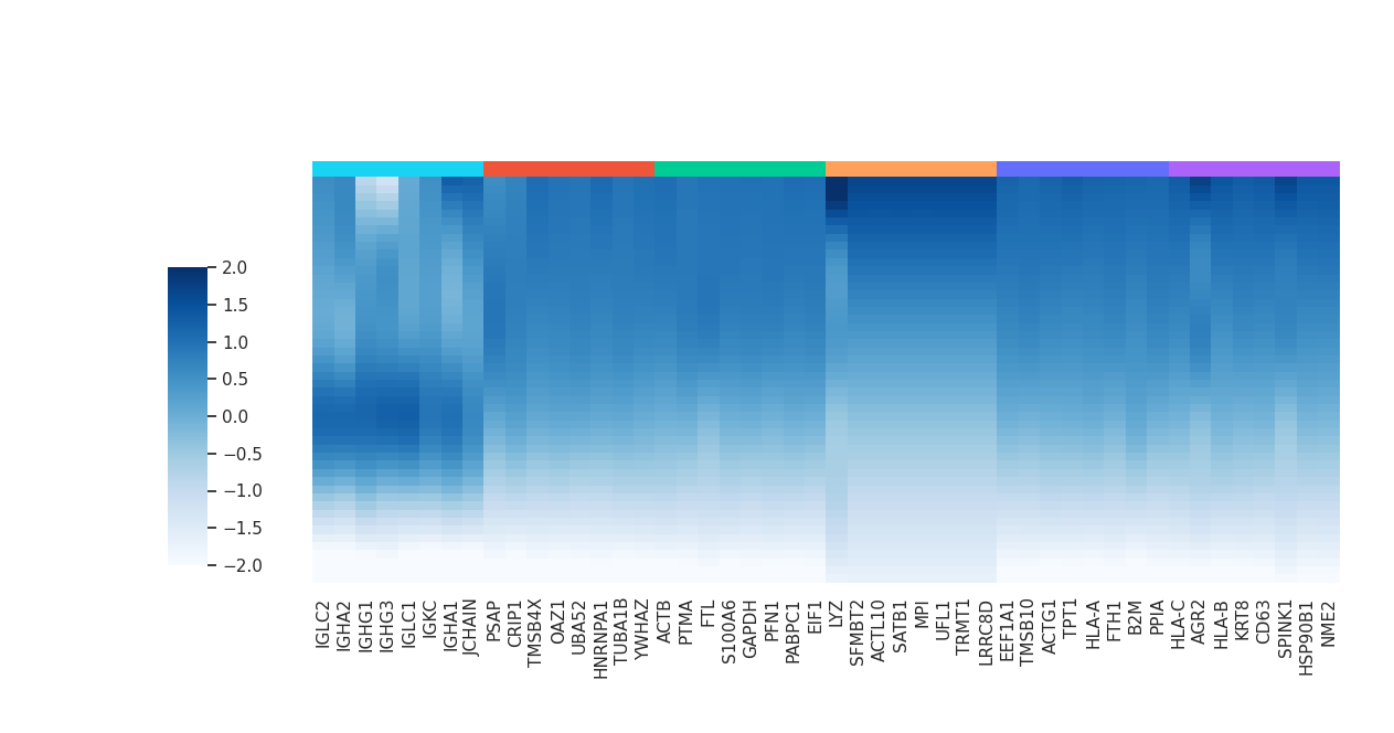
We can optionally remove ribosomal and mitochondrial genes from the analysis to reduce background noise and focus on biologically relevant communication response genes.
import re
pattern = re.compile(r'^(RPL|RPS|MT\-|NDU|CO|ATP5)')
mask = ~df_deg.index.to_series().str.match(pattern)
df_deg = df_deg[mask].copy()

df_deg_clus, df_yhat_clus = mc.tl.communication_responseGenes_cluster(df_deg.iloc[:,:3], df_yhat, deg_clustering_res=0.3)
mc.pl.plot_communication_responseGenes(df_deg = df_deg_clus,
                                       df_yhat = df_yhat_clus,
                                       top_ngene_per_cluster = 8,
                                       colormap = 'Blues',
                                       color_range = (-2,2),
                                       font_scale = 1,
                                       figsize = (12,6))
kegg_result = mc.tl.communication_responseGenes_keggEnrich(
    gene_list = df_deg[df_deg['pvalue'] < 0.05].index.tolist(),
    gene_sets = "KEGG_2021_Human",
    organism = "Human"
)
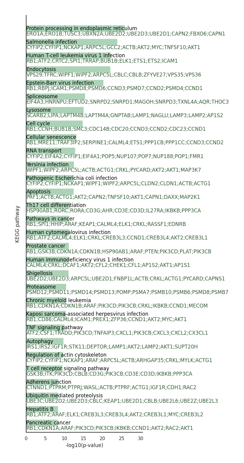
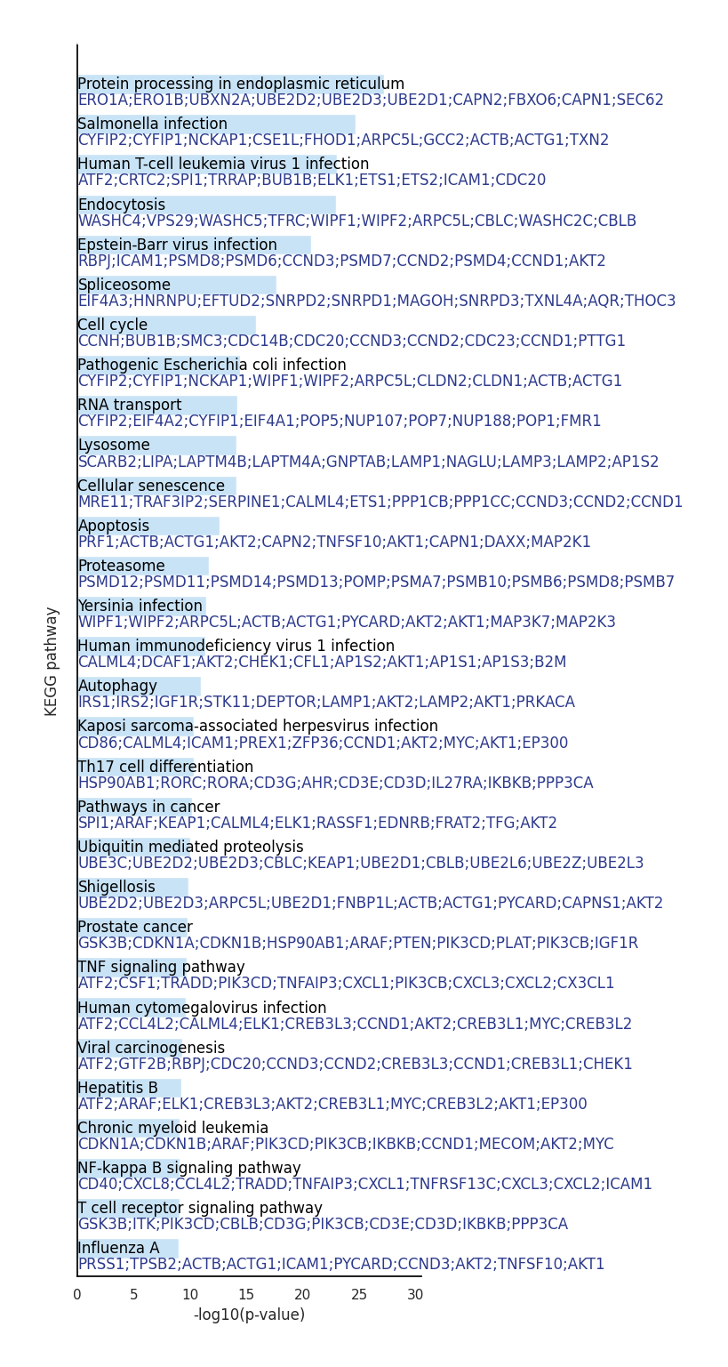
We can visualize top 30 KEGG pathway in these response genes.
mc.pl.plot_communication_responseGenes_keggEnrich(df_result = kegg_result,
                                                  show_term_order = range(30),
                                                  cmap = 'blue',
                                                  maxshow_gene = 10,
                                                  organism = "Human",
                                                  figsize = (5,18))
<Axes: xlabel='-log10(p-value)', ylabel='KEGG pathway'>
Aspartate Metabolism
metapathway_name = 'Aspartate Metabolism'
df_deg, df_yhat = mc.tl.communication_responseGenes(adata = adata,
                                                    adata_raw = adata_raw,
                                                    database_name = 'MetaChatDB',
                                                    metapathway_name = metapathway_name,
                                                    group_name = 'tissue_type',
                                                    summary = 'receiver')
100%|██████████| 100/100 [00:09<00:00, 10.52/s]
  |                                                  | 0 % ~calculating   |+                                                 | 1 % ~06m 39s       |+                                                 | 2 % ~06m 47s       |++                                                | 3 % ~06m 40s       |++                                                | 4 % ~06m 32s       |+++                                               | 5 % ~06m 22s       |+++                                               | 6 % ~06m 16s       |++++                                              | 7 % ~06m 16s       |++++                                              | 8 % ~06m 15s       |+++++                                             | 9 % ~06m 10s       |+++++                                             | 10% ~06m 09s       |++++++                                            | 11% ~06m 09s       |++++++                                            | 12% ~06m 24s       |+++++++                                           | 13% ~06m 21s       |+++++++                                           | 14% ~06m 18s       |++++++++                                          | 15% ~06m 13s       |++++++++                                          | 16% ~06m 11s       |+++++++++                                         | 17% ~06m 09s       |+++++++++                                         | 18% ~06m 07s       |++++++++++                                        | 19% ~06m 04s       |++++++++++                                        | 20% ~06m 00s       |+++++++++++                                       | 21% ~05m 56s       |+++++++++++                                       | 22% ~05m 52s       |++++++++++++                                      | 23% ~05m 50s       |++++++++++++                                      | 24% ~05m 50s       |+++++++++++++                                     | 25% ~05m 48s       |+++++++++++++                                     | 26% ~05m 44s       |++++++++++++++                                    | 27% ~05m 42s       |++++++++++++++                                    | 28% ~05m 38s       |+++++++++++++++                                   | 29% ~05m 34s       |+++++++++++++++                                   | 30% ~05m 30s       |++++++++++++++++                                  | 31% ~05m 26s       |++++++++++++++++                                  | 32% ~05m 23s       |+++++++++++++++++                                 | 33% ~05m 38s       |+++++++++++++++++                                 | 34% ~05m 33s       |++++++++++++++++++                                | 35% ~05m 29s       |++++++++++++++++++                                | 36% ~05m 24s       |+++++++++++++++++++                               | 37% ~05m 20s       |+++++++++++++++++++                               | 38% ~05m 15s       |++++++++++++++++++++                              | 39% ~05m 11s       |++++++++++++++++++++                              | 40% ~05m 07s       |+++++++++++++++++++++                             | 41% ~05m 02s       |+++++++++++++++++++++                             | 42% ~04m 57s       |++++++++++++++++++++++                            | 43% ~04m 54s       |++++++++++++++++++++++                            | 44% ~04m 49s       |+++++++++++++++++++++++                           | 45% ~04m 45s       |+++++++++++++++++++++++                           | 46% ~04m 40s       |++++++++++++++++++++++++                          | 47% ~04m 35s       |++++++++++++++++++++++++                          | 48% ~04m 30s       |+++++++++++++++++++++++++                         | 49% ~04m 25s       |+++++++++++++++++++++++++                         | 50% ~04m 21s       |++++++++++++++++++++++++++                        | 51% ~04m 16s       |++++++++++++++++++++++++++                        | 52% ~04m 11s       |+++++++++++++++++++++++++++                       | 53% ~04m 06s       |+++++++++++++++++++++++++++                       | 54% ~04m 01s       |++++++++++++++++++++++++++++                      | 55% ~03m 56s       |++++++++++++++++++++++++++++                      | 56% ~03m 51s       |+++++++++++++++++++++++++++++                     | 57% ~03m 46s       |+++++++++++++++++++++++++++++                     | 58% ~03m 41s       |++++++++++++++++++++++++++++++                    | 59% ~03m 36s       |++++++++++++++++++++++++++++++                    | 60% ~03m 31s       |+++++++++++++++++++++++++++++++                   | 61% ~03m 26s       |+++++++++++++++++++++++++++++++                   | 62% ~03m 21s       |++++++++++++++++++++++++++++++++                  | 63% ~03m 16s       |++++++++++++++++++++++++++++++++                  | 64% ~03m 11s       |+++++++++++++++++++++++++++++++++                 | 65% ~03m 06s       |+++++++++++++++++++++++++++++++++                 | 66% ~03m 01s       |++++++++++++++++++++++++++++++++++                | 67% ~02m 55s       |++++++++++++++++++++++++++++++++++                | 68% ~02m 50s       |+++++++++++++++++++++++++++++++++++               | 69% ~02m 45s       |+++++++++++++++++++++++++++++++++++               | 70% ~02m 40s       |++++++++++++++++++++++++++++++++++++              | 71% ~02m 35s       |++++++++++++++++++++++++++++++++++++              | 72% ~02m 30s       |+++++++++++++++++++++++++++++++++++++             | 73% ~02m 24s       |+++++++++++++++++++++++++++++++++++++             | 74% ~02m 19s       |++++++++++++++++++++++++++++++++++++++            | 75% ~02m 14s       |++++++++++++++++++++++++++++++++++++++            | 76% ~02m 09s       |+++++++++++++++++++++++++++++++++++++++           | 77% ~02m 04s       |+++++++++++++++++++++++++++++++++++++++           | 78% ~01m 58s       |++++++++++++++++++++++++++++++++++++++++          | 79% ~01m 53s       |++++++++++++++++++++++++++++++++++++++++          | 80% ~01m 48s       |+++++++++++++++++++++++++++++++++++++++++         | 81% ~01m 43s       |+++++++++++++++++++++++++++++++++++++++++         | 82% ~01m 37s       |++++++++++++++++++++++++++++++++++++++++++        | 83% ~01m 32s       |++++++++++++++++++++++++++++++++++++++++++        | 84% ~01m 27s       |+++++++++++++++++++++++++++++++++++++++++++       | 85% ~01m 21s       |+++++++++++++++++++++++++++++++++++++++++++       | 86% ~01m 16s       |++++++++++++++++++++++++++++++++++++++++++++      | 87% ~01m 11s       |++++++++++++++++++++++++++++++++++++++++++++      | 88% ~01m 05s       |+++++++++++++++++++++++++++++++++++++++++++++     | 89% ~60s           |+++++++++++++++++++++++++++++++++++++++++++++     | 90% ~54s           |++++++++++++++++++++++++++++++++++++++++++++++    | 91% ~49s           |++++++++++++++++++++++++++++++++++++++++++++++    | 92% ~44s           |+++++++++++++++++++++++++++++++++++++++++++++++   | 93% ~38s           |+++++++++++++++++++++++++++++++++++++++++++++++   | 94% ~33s           |++++++++++++++++++++++++++++++++++++++++++++++++  | 95% ~27s           |++++++++++++++++++++++++++++++++++++++++++++++++  | 96% ~22s           |+++++++++++++++++++++++++++++++++++++++++++++++++ | 97% ~16s           |+++++++++++++++++++++++++++++++++++++++++++++++++ | 98% ~11s           |++++++++++++++++++++++++++++++++++++++++++++++++++| 99% ~05s           |++++++++++++++++++++++++++++++++++++++++++++++++++| 100% elapsed=09m 07s
2 parameter combinations, 2 use sequential method, 2 use subsampling method
Running Clustering on Parameter Combinations...
done.
import re
pattern = re.compile(r'^(RPL|RPS|MT\-|NDU|CO|ATP5)')
mask = ~df_deg.index.to_series().str.match(pattern)
df_deg = df_deg[mask].copy()

df_deg_clus, df_yhat_clus = mc.tl.communication_responseGenes_cluster(df_deg.iloc[:,:3], df_yhat, deg_clustering_res=0.3)
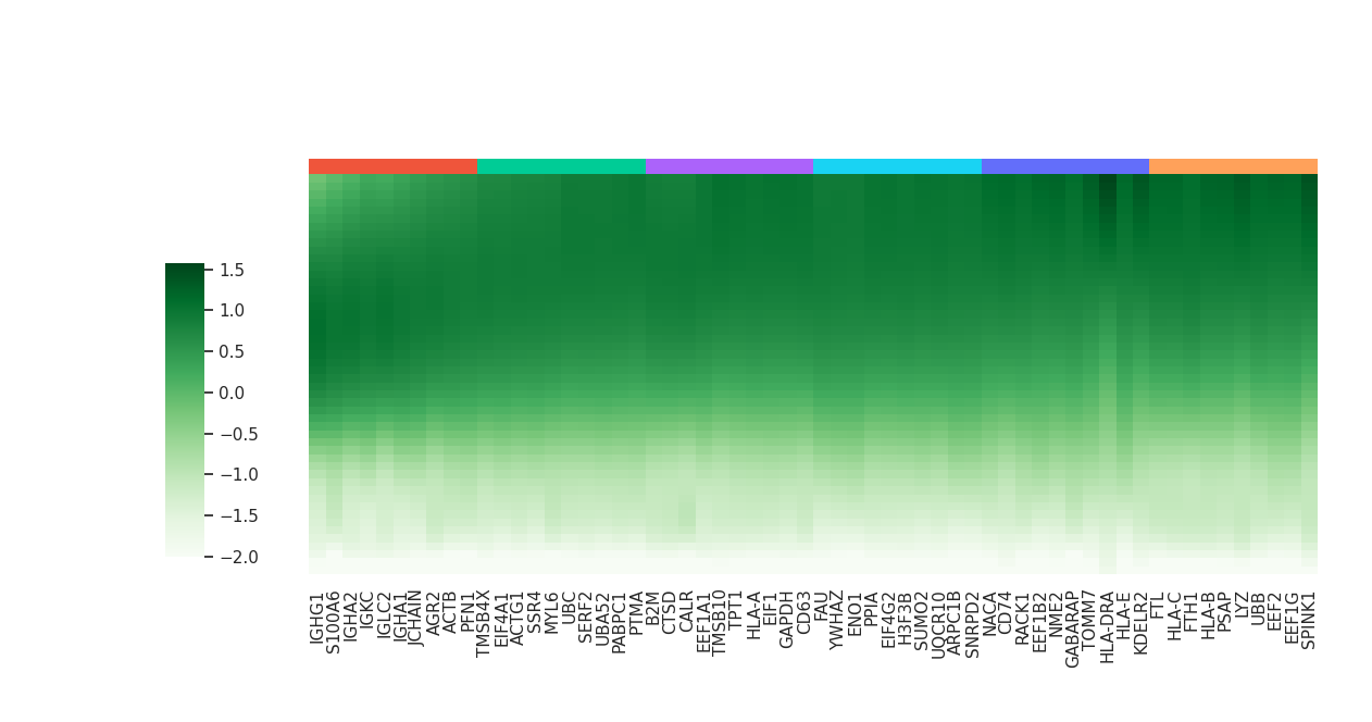
mc.pl.plot_communication_responseGenes(df_deg = df_deg_clus,
                                       df_yhat = df_yhat_clus,
                                       top_ngene_per_cluster = 10,
                                       colormap = 'Greens',
                                       color_range = (-2,2),
                                       font_scale = 1,
                                       figsize = (12,6))
kegg_result = mc.tl.communication_responseGenes_keggEnrich(
    gene_list = df_deg[df_deg['pvalue'] < 0.05].index.tolist(),
    gene_sets = "KEGG_2021_Human",
    organism = "Human"
)
mc.pl.plot_communication_responseGenes_keggEnrich(df_result = kegg_result,
                                                  show_term_order = range(30),
                                                  cmap = 'green',
                                                  maxshow_gene = 10,
                                                  organism = "Human",
                                                  figsize = (5,18))
<Axes: xlabel='-log10(p-value)', ylabel='KEGG pathway'>