Estimating spatial metabolomics from spatial transcriptomics using Compass

Brief introduction

In this tutorial, we demonstrate how to estimate spatial metabolomics maps from spatial transcriptomics datasets using Compass [Wagner et.al, 2021]. These inferred metabolite fluxes can then be integrated into MetaChat to infer metabolic cell communication (MCC).

Compass is a flux-balance-analysis (FBA)–based computational framework designed to infer cellular metabolic states from single-cell RNA sequencing data. It translates gene-expression levels of metabolic-enzyme-coding genes into reaction penalty scores, builds a constraint-based model of the metabolic network, and solves a set of linear programs to compute a score for every reaction in each cell.

The Compass algorithm is capable of estimating the abundance of around 429 different metabolites, offering a broader metabolite coverage compared to many alternative tools. However, this richer output comes at the cost of longer computational runtimes, so users should plan accordingly.

Installation

You can follow the guideline of installation from tutorials of Compass.

Create an independent environment

mamba create -n compass python=3.10
mamba activate compass

Install requirements:

python -m pip install numpy
python -m pip install git+https://github.com/wagnerlab-berkeley/Compass.git --upgrade

You can test if compass is sucessfully installed:

compass -h

The Compass framework uses the Gurobi Optimizer (a high-performance linear/linear-programming solver) to compute penalized reaction-scores by solving constrained optimization problems for each cell. To support academic research, Gurobi offers free full-featured academic licenses for faculty, students, and researchers at degree-granting institutions—these can be requested via their official academic program webpage.

If you sucessfully get the license, you can download the gurobi.lic file from the web license manager. Next, you will activate compass through:

compass --set-license <PATH_TO_LICENSE>

Usage

We use the Visium HD dataset of mouse small intestine, which also can be download from zenodo.

# Importing packages
import os
import scanpy as sc
import anndata as ad
import metachat as mc

# Setting your work directory
os.chdir("/home/project/metachat_packages/")

Import raw datasets of spatial transcritomics.

adata_RNA = sc.read('datasets/mouse_small_intestine/adata_16um_subset_rna_raw.h5ad')

The data should be normalized and log-transformed (log1p) before running Compass.

adata_RNA.var_names_make_unique()
adata_RNA.raw = adata_RNA
sc.pp.normalize_total(adata_RNA, inplace=True, target_sum=1e5)
sc.pp.log1p(adata_RNA)

adata_RNA

AnnData object with n_obs × n_vars = 8531 × 19059
    obs: 'in_tissue', 'array_row', 'array_col', 'location_id', 'region', 'Cluster'
    var: 'gene_ids', 'feature_types', 'genome'
    uns: 'Cluster_colors', 'spatial', 'spatialdata_attrs', 'log1p'
    obsm: 'spatial'

adata_RNA.write('datasets/mouse_small_intestine/adata_16um_subset_rna_normalized.h5ad')

Then, you can run compass on that normalized datasets in the compass environment.

compass --data <path to adata_16um_subset_rna_normalized.h5ad> \ 
        --num-processes 128 \ 
        --species mus_musculus \  # if human, homo_sapines
        --model RECON2_mat \
        --output-dir <path to output folder> \
        --temp-dir <path to output folder> \
        --calc-metabolites \  # Please select open because we need the abundance of metabolites.

The output includes reactions.tsv, secretions.tsv and uptake.tsv. We will use secretions.tsv as metabolite abundance and integrate it with the spatial transcriptomics data. Note that metabolites ending with [e] represent extracellular metabolites, which can be secreted or exchanged across the cell.

adata_META, _ = mc.pp.generate_adata_met_compass(data_path="datasets/mouse_small_intestine/compass_secretions.tsv")

Note

When comparing two or more datasets, it is crucial to manually adjust the baseline parameter in mc.pp.generate_adata_met_compass to ensure that all datasets share the same baseline value. This guarantees the comparability of normalized metabolite intensities across datasets.

A practical workflow is as follows:

1. Run generate_adata_met_compass separately on each dataset without specifying baseline:

   adata_A, baseline_A = mc.pp.generate_adata_met_compass(“dataset_A.tsv”) adata_B, baseline_B = mc.pp.generate_adata_met_compass(“dataset_B.tsv”)

2. Compare the two baseline values and choose the smaller one:

   common_baseline = min(baseline_A, baseline_B)

3. Re-run the function for both datasets using the same common_baseline:

   adata_A, _ = mc.pp.generate_adata_met_compass(“dataset_A.tsv”, baseline=common_baseline) adata_B, _ = mc.pp.generate_adata_met_compass(“dataset_B.tsv”, baseline=common_baseline)

This ensures that the processed metabolite matrices are on the same normalization scale and directly comparable across conditions.

adata_META

AnnData object with n_obs × n_vars = 8531 × 429

Then, we combine the spatial transcriptomics and metabolomics data.

adata_combined = ad.concat([adata_RNA, adata_META], axis=1, join="outer")
adata_combined.obs = adata_RNA.obs.copy()
adata_combined.uns = adata_RNA.uns.copy()
adata_combined.obsm = adata_RNA.obsm.copy()

adata_combined

AnnData object with n_obs × n_vars = 8531 × 19488
    obs: 'in_tissue', 'array_row', 'array_col', 'location_id', 'region', 'Cluster'
    var: 'gene_ids', 'feature_types', 'genome'
    uns: 'Cluster_colors', 'spatial', 'spatialdata_attrs', 'log1p'
    obsm: 'spatial'

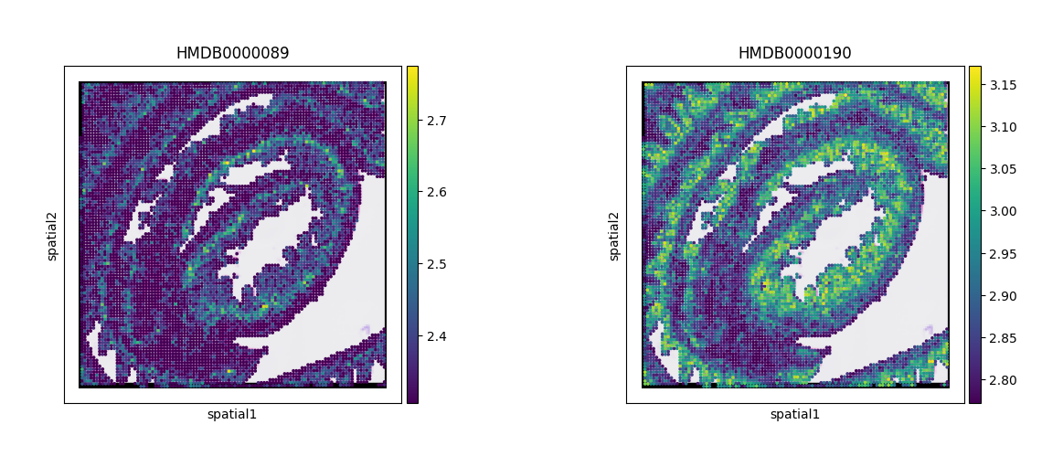
At this stage, we can visualize cytidine and lactate as examples, using their corresponding HMDB IDs.

sc.pl.spatial(adata_combined, color=["HMDB0000089","HMDB0000190"])