Downstream analysis on spatial multi-omics data of mouse brain with Parkinson’s disease
In this tutorial, we will perform downstream analysis of spatial multi-omics data from the mouse brain with Parkinson’s disease, including identification of MCC flow, group-level MCC, MCC remodelling in receiver cells.
# Importing packages
import os
import metachat as mc
import scanpy as sc

import matplotlib.pyplot as plt
from matplotlib import rcParams
rcParams['pdf.fonttype'] = 42
import warnings
warnings.filterwarnings("ignore", category=FutureWarning)
# Setting your work dictionary
os.chdir("/home/project/metachat_packages/")
Import MetaChat results
We manually annotated the MetaChat result using Napari, dividing the left hemisphere as “Intact” and the right hemisphere as “Lesion”. For convenience, we will directly import the annotated h5ad.
adata = sc.read('datasets/mouse_brain_parkinson/metachat_result_divided.h5ad')
The original output of MetaChat provides MCC signals for each individual metabolite–sensor pair.
Here, we use mc.tl.summary_communication to summarize the overall MCC activity associated with specific metabolites (e.g., dopamine and norepinephrine), aggregating their communication strengths across all corresponding sensors.
sum_metabolites = ['HMDB0000216', 'HMDB0000073']
mc.tl.summary_communication(adata = adata,
                            database_name = 'MetaChatDB',
                            sum_metabolites = sum_metabolites)
MCC flow
Then, we can compute the vector field of MCC flow using mc.tl.communication_flow, which estimates the spatial directionality and magnitude of MCC based on the summarized metabolite signals.
mc.tl.communication_flow(adata = adata,
                         database_name = 'MetaChatDB',
                         sum_metabolites = sum_metabolites,
                         k = 5)
The output vector fields are saved in adata.obsm, e.g., 'MetaChat-vf-MetaChatDB-sender-HMDB0000216' and 'MetaChat-vf-MetaChatDB-receiver-HMDB0000216', corresponding to the sender and receiver flows of each metabolite.
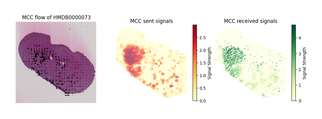
HMDB0000073: Dopamine
metabolite_name = "HMDB0000073"
fig, ax = plt.subplots(1, 3, figsize=(12,4))
pl1 = mc.pl.plot_communication_flow(adata = adata,
                                    database_name = 'MetaChatDB',
                                    metabolite_name = metabolite_name,
                                    plot_method = 'grid',
                                    background = 'image',
                                    summary = 'sender',
                                    ndsize = 3,
                                    normalize_v_quantile = 0.995,
                                    grid_density = 0.5,
                                    title = f'MCC flow of {metabolite_name}',
                                    ax = ax[0])
ax[0].set_box_aspect(1)

pl2 = mc.pl.plot_communication_flow(adata = adata,
                                    database_name = 'MetaChatDB',
                                    metabolite_name = metabolite_name,
                                    plot_method = None,
                                    background = 'summary',
                                    summary = 'sender',
                                    cmap = 'YlOrRd',
                                    ndsize = 5,
                                    normalize_v_quantile = 0.995,
                                    title = 'MCC sent signals',
                                    ax = ax[1])
ax[1].set_box_aspect(1)

pl3 = mc.pl.plot_communication_flow(adata = adata,
                                    database_name = 'MetaChatDB',
                                    metabolite_name = metabolite_name,
                                    plot_method = None,
                                    background = 'summary',
                                    summary = 'receiver',
                                    cmap = 'YlGn',
                                    ndsize = 5,
                                    normalize_v_quantile = 0.995,
                                    title = 'MCC received signals',
                                    ax = ax[2])
ax[2].set_box_aspect(1)
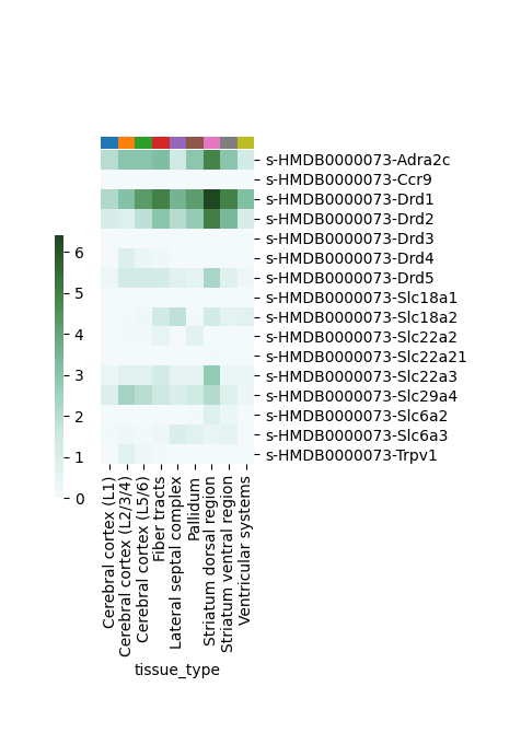
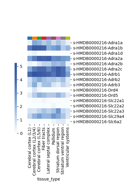
We can visualize which metabolite–sensor pairs contribute most to the overall MCC signals of a specific metabolite across tissue types using mc.pl.plot_MSpair_contribute_group.
mc.pl.plot_MSpair_contribute_group(adata = adata,
                                   database_name = 'MetaChatDB',
                                   group_name = 'tissue_type',
                                   metabolite_name = metabolite_name,
                                   summary = 'sender',
                                   cmap = 'green',
                                   figsize = (4,6))
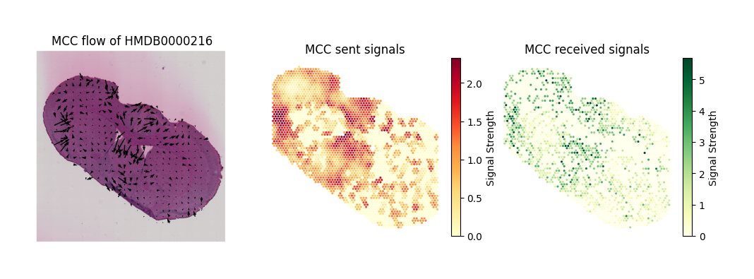
HMDB0000216: Norepinephrine
metabolite_name = "HMDB0000216"
fig, ax = plt.subplots(1, 3, figsize=(12,4))
pl1 = mc.pl.plot_communication_flow(adata = adata,
                                    database_name = 'MetaChatDB',
                                    metabolite_name = metabolite_name,
                                    plot_method = 'grid',
                                    background = 'image',
                                    summary = 'sender',
                                    ndsize = 3,
                                    normalize_v_quantile = 0.995,
                                    grid_density = 0.5,
                                    title = f'MCC flow of {metabolite_name}',
                                    ax = ax[0])
ax[0].set_box_aspect(1)

pl2 = mc.pl.plot_communication_flow(adata = adata,
                                    database_name = 'MetaChatDB',
                                    metabolite_name = metabolite_name,
                                    plot_method = None,
                                    background = 'summary',
                                    summary = 'sender',
                                    cmap = 'YlOrRd',
                                    ndsize = 5,
                                    normalize_v_quantile = 0.995,
                                    title = 'MCC sent signals',
                                    ax = ax[1])
ax[1].set_box_aspect(1)

pl3 = mc.pl.plot_communication_flow(adata = adata,
                                    database_name = 'MetaChatDB',
                                    metabolite_name = metabolite_name,
                                    plot_method = None,
                                    background = 'summary',
                                    summary = 'receiver',
                                    cmap = 'YlGn',
                                    ndsize = 5,
                                    normalize_v_quantile = 0.995,
                                    title = 'MCC received signals',
                                    ax = ax[2])
ax[2].set_box_aspect(1)
mc.pl.plot_MSpair_contribute_group(adata = adata,
                                   database_name = 'MetaChatDB',
                                   group_name = 'tissue_type',
                                   metabolite_name = metabolite_name,
                                   summary = 'sender',
                                   cmap = 'blue',
                                   figsize = (4,6))
MCC remodelling in receiver cells
In the next step, we aim to identify response genes in receiver cells. To do this, we provide the corresponding raw RNA data (adata_raw) as reference, which allows MetaChat to estimate transcriptional changes associated with signaling activity.
adata_raw = sc.read('datasets/mouse_brain_parkinson/adata_RNA_raw.h5ad')
HMDB0000073: Dopamine
The function mc.tl.communication_responseGenes supports identifying response genes within a defined spatial subset of the tissue, allowing users to focus on specific regions or cell groups where the received signal is most relevant.
metabolite_name = 'HMDB0000073'
df_deg, df_yhat = mc.tl.communication_responseGenes(adata = adata,
                                                    adata_raw = adata_raw,
                                                    database_name = 'MetaChatDB',
                                                    metabolite_name = metabolite_name,
                                                    subgroup = ['Striatum dorsal region', 'Striatum ventral region'],
                                                    group_name = 'tissue_type',
                                                    summary = 'receiver')
100%|██████████| 100/100 [00:13<00:00, 7.31/s]
  |                                                  | 0 % ~calculating   |+                                                 | 1 % ~03m 08s       |+                                                 | 2 % ~03m 04s       |++                                                | 3 % ~02m 60s       |++                                                | 4 % ~02m 60s       |+++                                               | 5 % ~02m 59s       |+++                                               | 6 % ~03m 26s       |++++                                              | 7 % ~03m 28s       |++++                                              | 8 % ~03m 46s       |+++++                                             | 9 % ~03m 46s       |+++++                                             | 10% ~03m 39s       |++++++                                            | 11% ~03m 32s       |++++++                                            | 12% ~03m 27s       |+++++++                                           | 13% ~03m 30s       |+++++++                                           | 14% ~03m 29s       |++++++++                                          | 15% ~03m 25s       |++++++++                                          | 16% ~03m 28s       |+++++++++                                         | 17% ~03m 26s       |+++++++++                                         | 18% ~03m 24s       |++++++++++                                        | 19% ~03m 20s       |++++++++++                                        | 20% ~03m 21s       |+++++++++++                                       | 21% ~03m 24s       |+++++++++++                                       | 22% ~03m 19s       |++++++++++++                                      | 23% ~03m 28s       |++++++++++++                                      | 24% ~03m 24s       |+++++++++++++                                     | 25% ~03m 23s       |+++++++++++++                                     | 26% ~03m 19s       |++++++++++++++                                    | 27% ~03m 15s       |++++++++++++++                                    | 28% ~03m 13s       |+++++++++++++++                                   | 29% ~03m 09s       |+++++++++++++++                                   | 30% ~03m 06s       |++++++++++++++++                                  | 31% ~03m 02s       |++++++++++++++++                                  | 32% ~03m 06s       |+++++++++++++++++                                 | 33% ~03m 02s       |+++++++++++++++++                                 | 34% ~02m 58s       |++++++++++++++++++                                | 35% ~02m 57s       |++++++++++++++++++                                | 36% ~02m 54s       |+++++++++++++++++++                               | 37% ~02m 50s       |+++++++++++++++++++                               | 38% ~02m 47s       |++++++++++++++++++++                              | 39% ~02m 44s       |++++++++++++++++++++                              | 40% ~02m 40s       |+++++++++++++++++++++                             | 41% ~02m 38s       |+++++++++++++++++++++                             | 42% ~02m 34s       |++++++++++++++++++++++                            | 43% ~02m 31s       |++++++++++++++++++++++                            | 44% ~02m 30s       |+++++++++++++++++++++++                           | 45% ~02m 28s       |+++++++++++++++++++++++                           | 46% ~02m 26s       |++++++++++++++++++++++++                          | 47% ~02m 23s       |++++++++++++++++++++++++                          | 48% ~02m 20s       |+++++++++++++++++++++++++                         | 49% ~02m 18s       |+++++++++++++++++++++++++                         | 50% ~02m 15s       |++++++++++++++++++++++++++                        | 51% ~02m 13s       |++++++++++++++++++++++++++                        | 52% ~02m 11s       |+++++++++++++++++++++++++++                       | 53% ~02m 08s       |+++++++++++++++++++++++++++                       | 54% ~02m 08s       |++++++++++++++++++++++++++++                      | 55% ~02m 05s       |++++++++++++++++++++++++++++                      | 56% ~02m 02s       |+++++++++++++++++++++++++++++                     | 57% ~02m 01s       |+++++++++++++++++++++++++++++                     | 58% ~02m 00s       |++++++++++++++++++++++++++++++                    | 59% ~01m 57s       |++++++++++++++++++++++++++++++                    | 60% ~01m 59s       |+++++++++++++++++++++++++++++++                   | 61% ~01m 56s       |+++++++++++++++++++++++++++++++                   | 62% ~01m 52s       |++++++++++++++++++++++++++++++++                  | 63% ~01m 50s       |++++++++++++++++++++++++++++++++                  | 64% ~01m 47s       |+++++++++++++++++++++++++++++++++                 | 65% ~01m 44s       |+++++++++++++++++++++++++++++++++                 | 66% ~01m 41s       |++++++++++++++++++++++++++++++++++                | 67% ~01m 37s       |++++++++++++++++++++++++++++++++++                | 68% ~01m 34s       |+++++++++++++++++++++++++++++++++++               | 69% ~01m 31s       |+++++++++++++++++++++++++++++++++++               | 70% ~01m 28s       |++++++++++++++++++++++++++++++++++++              | 71% ~01m 25s       |++++++++++++++++++++++++++++++++++++              | 72% ~01m 22s       |+++++++++++++++++++++++++++++++++++++             | 73% ~01m 19s       |+++++++++++++++++++++++++++++++++++++             | 74% ~01m 16s       |++++++++++++++++++++++++++++++++++++++            | 75% ~01m 12s       |++++++++++++++++++++++++++++++++++++++            | 76% ~01m 09s       |+++++++++++++++++++++++++++++++++++++++           | 77% ~01m 07s       |+++++++++++++++++++++++++++++++++++++++           | 78% ~01m 04s       |++++++++++++++++++++++++++++++++++++++++          | 79% ~01m 02s       |++++++++++++++++++++++++++++++++++++++++          | 80% ~59s           |+++++++++++++++++++++++++++++++++++++++++         | 81% ~56s           |+++++++++++++++++++++++++++++++++++++++++         | 82% ~53s           |++++++++++++++++++++++++++++++++++++++++++        | 83% ~50s           |++++++++++++++++++++++++++++++++++++++++++        | 84% ~47s           |+++++++++++++++++++++++++++++++++++++++++++       | 85% ~44s           |+++++++++++++++++++++++++++++++++++++++++++       | 86% ~42s           |++++++++++++++++++++++++++++++++++++++++++++      | 87% ~38s           |++++++++++++++++++++++++++++++++++++++++++++      | 88% ~35s           |+++++++++++++++++++++++++++++++++++++++++++++     | 89% ~32s           |+++++++++++++++++++++++++++++++++++++++++++++     | 90% ~29s           |++++++++++++++++++++++++++++++++++++++++++++++    | 91% ~26s           |++++++++++++++++++++++++++++++++++++++++++++++    | 92% ~23s           |+++++++++++++++++++++++++++++++++++++++++++++++   | 93% ~21s           |+++++++++++++++++++++++++++++++++++++++++++++++   | 94% ~18s           |++++++++++++++++++++++++++++++++++++++++++++++++  | 95% ~15s           |++++++++++++++++++++++++++++++++++++++++++++++++  | 96% ~12s           |+++++++++++++++++++++++++++++++++++++++++++++++++ | 97% ~09s           |+++++++++++++++++++++++++++++++++++++++++++++++++ | 98% ~06s           |++++++++++++++++++++++++++++++++++++++++++++++++++| 99% ~03s           |++++++++++++++++++++++++++++++++++++++++++++++++++| 100% elapsed=04m 52s
2 parameter combinations, 2 use sequential method, 2 use subsampling method
Running Clustering on Parameter Combinations...
done.
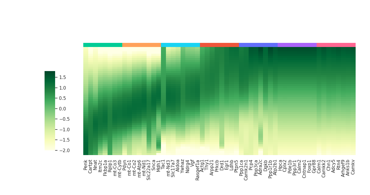
Next, we clustered the response genes based on their expression trends along the received signaling strength. This allows us to identify distinct transcriptional programs that are activated or suppressed in response to MCC signal.
df_deg_clus, df_yhat_clus = mc.tl.communication_responseGenes_cluster(df_deg.iloc[:,:3], df_yhat, deg_clustering_res=0.3)
mc.pl.plot_communication_responseGenes(
    df_deg = df_deg_clus,
    df_yhat = df_yhat_clus,
    top_ngene_per_cluster = 8,
    colormap = 'YlGn',
    color_range = (-2,2),
    font_scale = 1,
    figsize = (12,6),
    return_genes = False
)
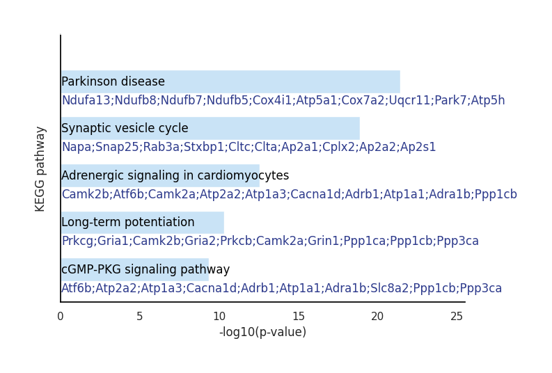
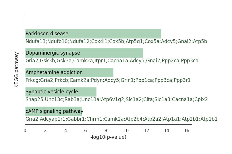
kegg_result = mc.tl.communication_responseGenes_keggEnrich(
    gene_list = df_deg[df_deg['pvalue'] < 0.05].index.tolist()[:1000],
    gene_sets = "KEGG_2019_Mouse",
    organism = "Mouse")
mc.pl.plot_communication_responseGenes_keggEnrich(
    df_result = kegg_result,
    show_term_order = [2,5,11,17,25],
    cmap = 'green',
    maxshow_gene = 10,
    organism = "Mouse",
    figsize = (7.5,5))
<Axes: xlabel='-log10(p-value)', ylabel='KEGG pathway'>
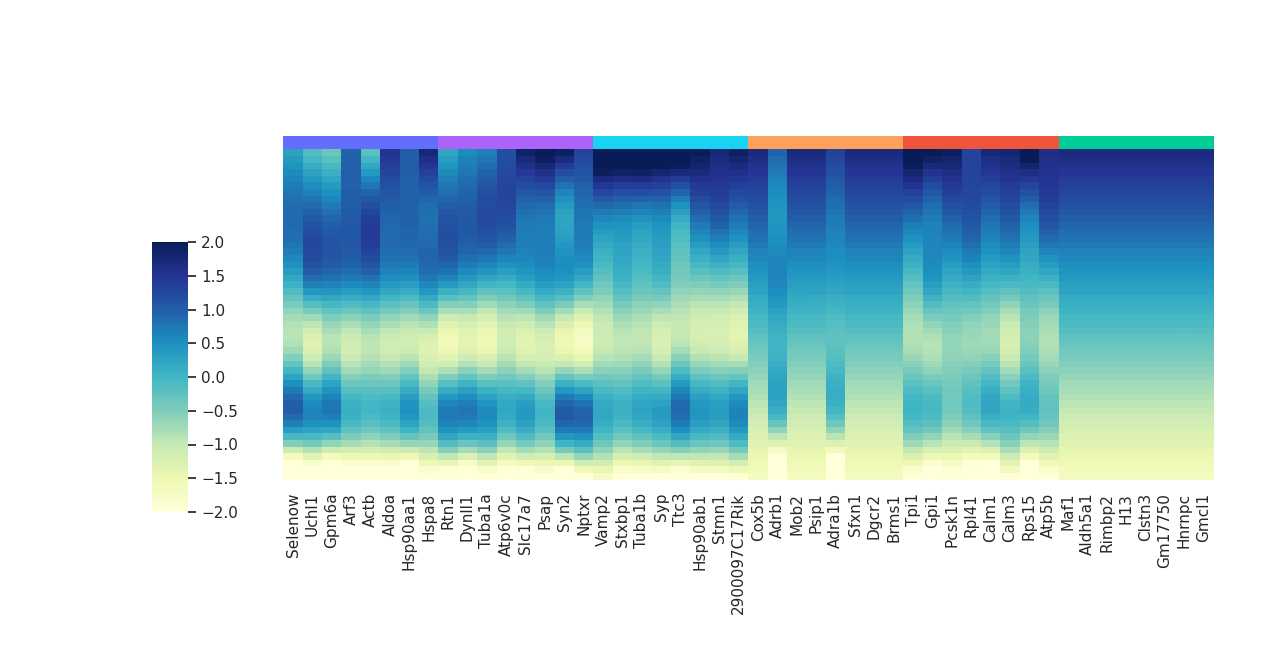
HMDB0000216: Norepinephrine
adata_raw = sc.read('datasets/mouse_brain_parkinson/adata_RNA_raw.h5ad')
metabolite_name = 'HMDB0000216'
df_deg, df_yhat = mc.tl.communication_responseGenes(
    adata = adata,
    adata_raw = adata_raw,
    database_name = 'MetaChatDB',
    metabolite_name = metabolite_name,
    subgroup = ['Cerebral cortex (L1)', 'Cerebral cortex (L2/3/4)', 'Cerebral cortex (L5/6)'],
    group_name = 'tissue_type',
    summary = 'receiver'
)
100%|██████████| 100/100 [00:12<00:00, 7.85/s]
  |                                                  | 0 % ~calculating   |+                                                 | 1 % ~03m 49s       |+                                                 | 2 % ~03m 37s       |++                                                | 3 % ~03m 55s       |++                                                | 4 % ~03m 55s       |+++                                               | 5 % ~04m 04s       |+++                                               | 6 % ~04m 26s       |++++                                              | 7 % ~04m 54s       |++++                                              | 8 % ~04m 45s       |+++++                                             | 9 % ~04m 43s       |+++++                                             | 10% ~04m 32s       |++++++                                            | 11% ~04m 28s       |++++++                                            | 12% ~04m 29s       |+++++++                                           | 13% ~05m 15s       |+++++++                                           | 14% ~05m 23s       |++++++++                                          | 15% ~05m 19s       |++++++++                                          | 16% ~05m 21s       |+++++++++                                         | 17% ~05m 19s       |+++++++++                                         | 18% ~05m 15s       |++++++++++                                        | 19% ~05m 05s       |++++++++++                                        | 20% ~05m 11s       |+++++++++++                                       | 21% ~05m 13s       |+++++++++++                                       | 22% ~05m 04s       |++++++++++++                                      | 23% ~05m 03s       |++++++++++++                                      | 24% ~04m 57s       |+++++++++++++                                     | 25% ~04m 57s       |+++++++++++++                                     | 26% ~04m 51s       |++++++++++++++                                    | 27% ~04m 44s       |++++++++++++++                                    | 28% ~04m 37s       |+++++++++++++++                                   | 29% ~04m 37s       |+++++++++++++++                                   | 30% ~04m 30s       |++++++++++++++++                                  | 31% ~04m 23s       |++++++++++++++++                                  | 32% ~04m 20s       |+++++++++++++++++                                 | 33% ~04m 14s       |+++++++++++++++++                                 | 34% ~04m 10s       |++++++++++++++++++                                | 35% ~04m 05s       |++++++++++++++++++                                | 36% ~04m 03s       |+++++++++++++++++++                               | 37% ~04m 01s       |+++++++++++++++++++                               | 38% ~03m 55s       |++++++++++++++++++++                              | 39% ~03m 49s       |++++++++++++++++++++                              | 40% ~03m 45s       |+++++++++++++++++++++                             | 41% ~03m 42s       |+++++++++++++++++++++                             | 42% ~03m 38s       |++++++++++++++++++++++                            | 43% ~03m 39s       |++++++++++++++++++++++                            | 44% ~03m 37s       |+++++++++++++++++++++++                           | 45% ~03m 33s       |+++++++++++++++++++++++                           | 46% ~03m 29s       |++++++++++++++++++++++++                          | 47% ~03m 26s       |++++++++++++++++++++++++                          | 48% ~03m 22s       |+++++++++++++++++++++++++                         | 49% ~03m 19s       |+++++++++++++++++++++++++                         | 50% ~03m 15s       |++++++++++++++++++++++++++                        | 51% ~03m 10s       |++++++++++++++++++++++++++                        | 52% ~03m 06s       |+++++++++++++++++++++++++++                       | 53% ~03m 03s       |+++++++++++++++++++++++++++                       | 54% ~03m 00s       |++++++++++++++++++++++++++++                      | 55% ~02m 58s       |++++++++++++++++++++++++++++                      | 56% ~02m 53s       |+++++++++++++++++++++++++++++                     | 57% ~02m 50s       |+++++++++++++++++++++++++++++                     | 58% ~02m 47s       |++++++++++++++++++++++++++++++                    | 59% ~02m 44s       |++++++++++++++++++++++++++++++                    | 60% ~02m 41s       |+++++++++++++++++++++++++++++++                   | 61% ~02m 37s       |+++++++++++++++++++++++++++++++                   | 62% ~02m 32s       |++++++++++++++++++++++++++++++++                  | 63% ~02m 27s       |++++++++++++++++++++++++++++++++                  | 64% ~02m 23s       |+++++++++++++++++++++++++++++++++                 | 65% ~02m 19s       |+++++++++++++++++++++++++++++++++                 | 66% ~02m 15s       |++++++++++++++++++++++++++++++++++                | 67% ~02m 10s       |++++++++++++++++++++++++++++++++++                | 68% ~02m 07s       |+++++++++++++++++++++++++++++++++++               | 69% ~02m 02s       |+++++++++++++++++++++++++++++++++++               | 70% ~01m 58s       |++++++++++++++++++++++++++++++++++++              | 71% ~01m 54s       |++++++++++++++++++++++++++++++++++++              | 72% ~01m 50s       |+++++++++++++++++++++++++++++++++++++             | 73% ~01m 46s       |+++++++++++++++++++++++++++++++++++++             | 74% ~01m 43s       |++++++++++++++++++++++++++++++++++++++            | 75% ~01m 39s       |++++++++++++++++++++++++++++++++++++++            | 76% ~01m 35s       |+++++++++++++++++++++++++++++++++++++++           | 77% ~01m 31s       |+++++++++++++++++++++++++++++++++++++++           | 78% ~01m 27s       |++++++++++++++++++++++++++++++++++++++++          | 79% ~01m 23s       |++++++++++++++++++++++++++++++++++++++++          | 80% ~01m 19s       |+++++++++++++++++++++++++++++++++++++++++         | 81% ~01m 15s       |+++++++++++++++++++++++++++++++++++++++++         | 82% ~01m 11s       |++++++++++++++++++++++++++++++++++++++++++        | 83% ~01m 07s       |++++++++++++++++++++++++++++++++++++++++++        | 84% ~01m 03s       |+++++++++++++++++++++++++++++++++++++++++++       | 85% ~60s           |+++++++++++++++++++++++++++++++++++++++++++       | 86% ~56s           |++++++++++++++++++++++++++++++++++++++++++++      | 87% ~52s           |++++++++++++++++++++++++++++++++++++++++++++      | 88% ~48s           |+++++++++++++++++++++++++++++++++++++++++++++     | 89% ~44s           |+++++++++++++++++++++++++++++++++++++++++++++     | 90% ~40s           |++++++++++++++++++++++++++++++++++++++++++++++    | 91% ~36s           |++++++++++++++++++++++++++++++++++++++++++++++    | 92% ~32s           |+++++++++++++++++++++++++++++++++++++++++++++++   | 93% ~28s           |+++++++++++++++++++++++++++++++++++++++++++++++   | 94% ~24s           |++++++++++++++++++++++++++++++++++++++++++++++++  | 95% ~20s           |++++++++++++++++++++++++++++++++++++++++++++++++  | 96% ~16s           |+++++++++++++++++++++++++++++++++++++++++++++++++ | 97% ~12s           |+++++++++++++++++++++++++++++++++++++++++++++++++ | 98% ~08s           |++++++++++++++++++++++++++++++++++++++++++++++++++| 99% ~04s           |++++++++++++++++++++++++++++++++++++++++++++++++++| 100% elapsed=06m 36s
2 parameter combinations, 2 use sequential method, 2 use subsampling method
Running Clustering on Parameter Combinations...
done.
df_deg_clus, df_yhat_clus = mc.tl.communication_responseGenes_cluster(df_deg.iloc[:,:3], df_yhat, deg_clustering_res=0.3)
mc.pl.plot_communication_responseGenes(
    df_deg = df_deg_clus,
    df_yhat = df_yhat_clus,
    top_ngene_per_cluster = 8,
    colormap = 'YlGnBu',
    color_range = (-2,2),
    font_scale = 1,
    figsize = (12,6),
    return_genes = False
)
kegg_result_subgroup = mc.tl.communication_responseGenes_keggEnrich(
    gene_list = df_deg[df_deg['pvalue'] < 0.05].index.tolist()[:1000],
    gene_sets = "KEGG_2019_Mouse",
    organism = "Mouse"
)
mc.pl.plot_communication_responseGenes_keggEnrich(
    df_result = kegg_result_subgroup,
    show_term_order = [3,5,7,10,14],
    cmap = 'blue',
    maxshow_gene = 10,
    organism = "Mouse",
    figsize = (7.5,5)
)
<Axes: xlabel='-log10(p-value)', ylabel='KEGG pathway'>